class: center, middle, inverse, title-slide # Basics of R Programming ### <br><br>Thiyanga S. Talagala, University of Sri Jayewardenepura ### SLAAS - Aug 28/29, 2021 --- <style type="text/css"> .remark-slide-content { font-size: 35px; } </style> <style type="text/css"> .remark-slide-content { font-size: 35px; } </style> <style> p.comment { background-color: #DBDBDB; padding: 10px; border: 1px solid black; margin-left: 25px; border-radius: 5px; font-style: italic; } </style> <style type="text/css"> h1, #TOC>ul>li { color: #1b9e77; font-weight: bold; } h2, #TOC>ul>ul>li { color: #1b9e77; #font-family: "Times"; font-weight: bold; } h3, #TOC>ul>ul>li { color: #00441b; #font-family: "Times"; font-weight: bold; } </style> .pull-left[ ## Data structures Way to **store and organize data** so that it can be used efficiently. ```r marks <- c(100, 40, 34, 97, 98) marks ``` ``` [1] 100 40 34 97 98 ``` ] -- .pull-right[ ## Functions Tell R to **do something** ```r mean(marks) ``` ``` [1] 73.8 ``` ```r summary(marks) ``` ``` Min. 1st Qu. Median Mean 3rd Qu. Max. 34.0 40.0 97.0 73.8 98.0 100.0 ``` ] --- ## Data structures <img src="ds.png" width="80%" /> Source: Ceballos and Cardiel, 2013 --- ## Creating vectors Syntax ```r vector_name <- c(element1, element2, element3) ``` Example ```r x <- c(5, 6, 3, 1, 100) x ``` ``` [1] 5 6 3 1 100 ``` --- ## Combine two vectors ```r p <- c(1, 2, 3) p ``` ``` [1] 1 2 3 ``` ```r q <- c(10, 20, 30) q ``` ``` [1] 10 20 30 ``` ```r r <- c(p, q) r ``` ``` [1] 1 2 3 10 20 30 ``` --- ## Vector with charactor elements ```r names <- c("USJ", "UM", "UC", "UJ") names ``` ``` [1] "USJ" "UM" "UC" "UJ" ``` ## Logical vector ```r result <- c(TRUE, FALSE, FALSE, TRUE, FALSE) result ``` ``` [1] TRUE FALSE FALSE TRUE FALSE ``` --- ## Simplifying vector creation ```r id <- 1:10 id ``` ``` [1] 1 2 3 4 5 6 7 8 9 10 ``` ```r treatment <- rep(1:3, each=2) treatment ``` ``` [1] 1 1 2 2 3 3 ``` Additional resources: https://hellor.netlify.app/2021/week1/l12021.html#62 --- ## Vector operations ```r x <- c(1, 2, 3) y <- c(10, 20, 30) x+y ``` ``` [1] 11 22 33 ``` ```r p <- c(100, 1000) x+p ``` ``` [1] 101 1002 103 ``` --- ## Data set <img src="excel.png" width="50%" /> --- ## Required R package ```r library(tidyverse) ``` ``` ── Attaching packages ─────────────────────────────────────── tidyverse 1.3.1 ── ``` ``` ✓ ggplot2 3.3.5 ✓ purrr 0.3.4 ✓ tibble 3.1.2 ✓ dplyr 1.0.7 ✓ tidyr 1.1.3 ✓ stringr 1.4.0 ✓ readr 1.4.0 ✓ forcats 0.5.1 ``` ``` ── Conflicts ────────────────────────────────────────── tidyverse_conflicts() ── x dplyr::filter() masks stats::filter() x dplyr::lag() masks stats::lag() ``` --- ## Create a tibble .pull-left[ <img src="excel.png" width="80%" /> ] .pull-right[ ```r marks <- c(90, 50, 20, 60) grade <- factor(c("A+", "C", "E", "B")) final <- tibble(Marks = marks, Grade = grade) final ``` ``` # A tibble: 4 x 2 Marks Grade <dbl> <fct> 1 90 A+ 2 50 C 3 20 E 4 60 B ``` ] --- ## Create a tibble ```r marks <- c(90, 50, 20, 60) grade <- factor(c("A+", "C", "E", "B"), * level = c("A+", "A", "B+", "B", "C", "D", "E")) final <- tibble(Marks = marks, Grade = grade) final ``` ``` # A tibble: 4 x 2 Marks Grade <dbl> <fct> 1 90 A+ 2 50 C 3 20 E 4 60 B ``` --- class: inverse, middle, center # Functions in R --- .pull-left[ # Data set: tibble ```r final ``` ``` # A tibble: 4 x 2 Marks Grade <dbl> <fct> 1 90 A+ 2 50 C 3 20 E 4 60 B ``` ] .pull-right[ ## Functions ```r summary(final) ``` ``` Marks Grade Min. :20.0 A+:1 1st Qu.:42.5 A :0 Median :55.0 B+:0 Mean :55.0 B :1 3rd Qu.:67.5 C :1 Max. :90.0 D :0 E :1 ``` ] --- ## Your Turn <img src="excel2.png" width="40%" /> <div class="countdown" id="timer_61296e5a" style="right:0;bottom:0;" data-warnwhen="0"> <code class="countdown-time"><span class="countdown-digits minutes">01</span><span class="countdown-digits colon">:</span><span class="countdown-digits seconds">00</span></code> </div> --- .pull-left[ <img src="excel2.png" width="70%" /> ] .pull-right[ ```r h <- c(100, 101, 102, 150, NA) w <- c(50, 60, 80, 43, 50) hwdata <- tibble(Height=h, Weight=w) hwdata ``` ``` # A tibble: 5 x 2 Height Weight <dbl> <dbl> 1 100 50 2 101 60 3 102 80 4 150 43 5 NA 50 ``` ] --- .pull-left[ ```r hwdata ``` ``` # A tibble: 5 x 2 Height Weight <dbl> <dbl> 1 100 50 2 101 60 3 102 80 4 150 43 5 NA 50 ``` ] .pull-right[ ```r summary(hwdata) ``` ``` Height Weight Min. :100.0 Min. :43.0 1st Qu.:100.8 1st Qu.:50.0 Median :101.5 Median :50.0 Mean :113.2 Mean :56.6 3rd Qu.:114.0 3rd Qu.:60.0 Max. :150.0 Max. :80.0 NA's :1 ``` ] --- .pull-left[ # Subsetting ```r hwdata ``` ``` # A tibble: 5 x 2 Height Weight <dbl> <dbl> 1 100 50 2 101 60 3 102 80 4 150 43 5 NA 50 ``` ```r hwdata[1, 1] ``` ``` # A tibble: 1 x 1 Height <dbl> 1 100 ``` ] .pull-right[ ```r hwdata[, 1] ``` ``` # A tibble: 5 x 1 Height <dbl> 1 100 2 101 3 102 4 150 5 NA ``` ```r hwdata[1, ] ``` ``` # A tibble: 1 x 2 Height Weight <dbl> <dbl> 1 100 50 ``` ```r hwdata$Height ``` ``` [1] 100 101 102 150 NA ``` ] --- # Help file .pull-left[ ```r hwdata$Weight ``` ``` [1] 50 60 80 43 50 ``` ```r mean(hwdata$Weight) ``` ``` [1] 56.6 ``` ] .pull-right[ ```r hwdata$Height ``` ``` [1] 100 101 102 150 NA ``` ```r mean(hwdata$Height) ``` ``` [1] NA ``` ] --- # Help file .pull-left[ ```r hwdata$Weight ``` ``` [1] 50 60 80 43 50 ``` ```r mean(hwdata$Weight) ``` ``` [1] 56.6 ``` ] .pull-right[ ```r hwdata$Height ``` ``` [1] 100 101 102 150 NA ``` ```r mean(hwdata$Height) ``` ``` [1] NA ``` ```r mean(hwdata$Height, na.rm=TRUE) ``` ``` [1] 113.25 ``` ] --- .pull-left[ # Help file ```r ?mean help(mean) ``` ] .pull-right[ <img src="help.png" width="170%" /> ] --- # Commenting ```r mean(hwdata$Height, na.rm=TRUE) # compute mean of height ``` ``` [1] 113.25 ``` --- # Some useful functions .pull-left[ ```r mean(hwdata$Weight) ``` ``` [1] 56.6 ``` ```r median(hwdata$Weight) ``` ``` [1] 50 ``` ```r sd(hwdata$Weight) ``` ``` [1] 14.41527 ``` ] .pull-right[ ```r sum(hwdata$Weight) ``` ``` [1] 283 ``` ```r length(hwdata$Weight) ``` ``` [1] 5 ``` ] --- ## Pipe operator (`%>%`) .pull-left[ ```r mean(hwdata$Weight) ``` ``` [1] 56.6 ``` ```r mean(hwdata$Height, na.rm=TRUE) ``` ``` [1] 113.25 ``` ] .pull-right[ ```r library(magrittr) hwdata$Weight %>% mean() ``` ``` [1] 56.6 ``` ```r hwdata$Height %>% mean(na.rm=TRUE) ``` ``` [1] 113.25 ``` ] --- ## Pipe operator (`%>%`) 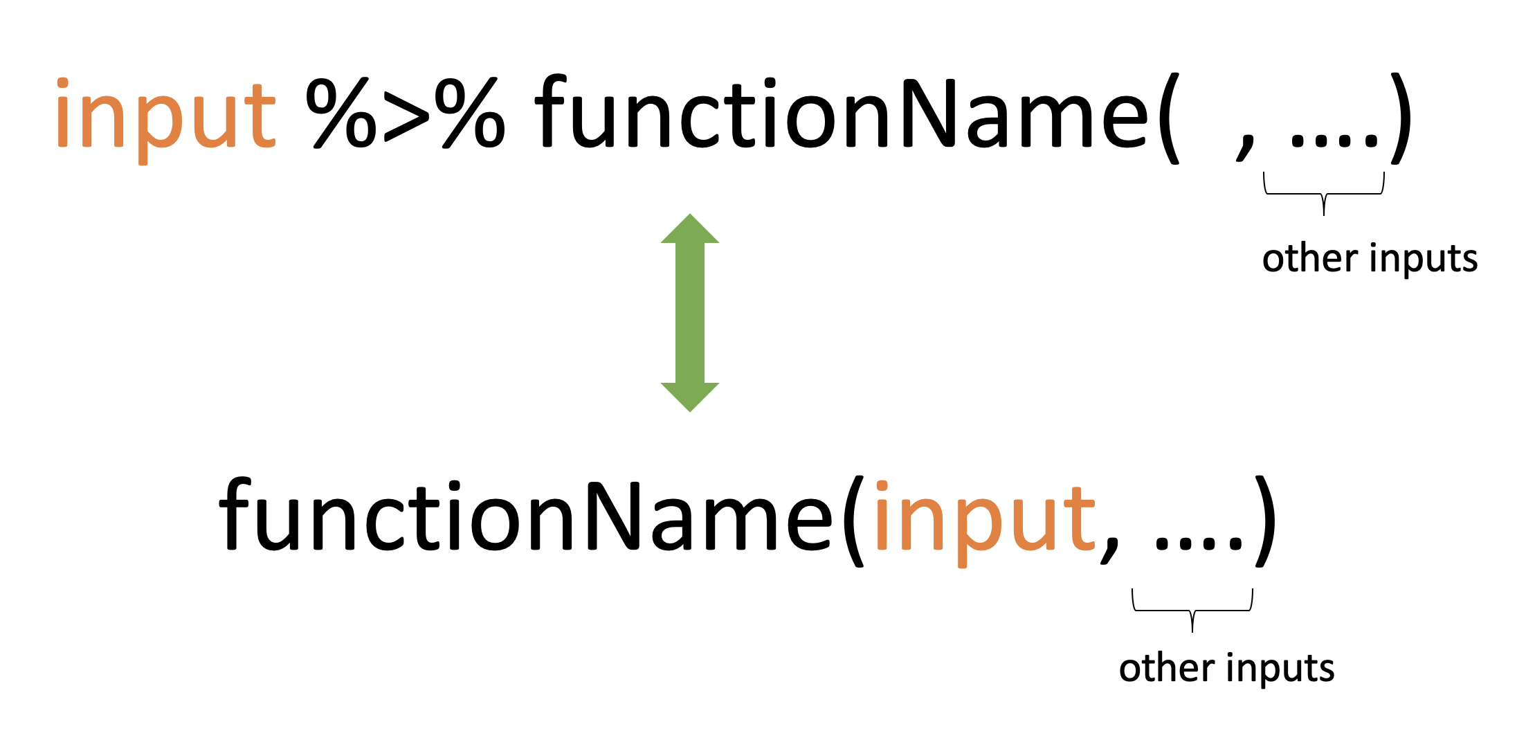 --- class: inverse, cover, middle # Recap ✅ Data structures and functions ✅ Factors ✅ Working with packages ✅ Create a tibble ✅ Help file ✅ Commenting