class: center, middle, inverse, title-slide # Basics of R Programming ### <br><br>Thiyanga S. Talagala, University of Sri Jayewardenepura ### IASSL - Feb 21/25, 2022 --- <style type="text/css"> .remark-slide-content { font-size: 35px; } </style> <style type="text/css"> .remark-slide-content { font-size: 35px; } </style> <style> p.comment { background-color: #DBDBDB; padding: 10px; border: 1px solid black; margin-left: 25px; border-radius: 5px; font-style: italic; } </style> <style type="text/css"> h1, #TOC>ul>li { color: #1b9e77; font-weight: bold; } h2, #TOC>ul>ul>li { color: #1b9e77; #font-family: "Times"; font-weight: bold; } h3, #TOC>ul>ul>li { color: #00441b; #font-family: "Times"; font-weight: bold; } </style> .pull-left[ ## Data structures Way to **store and organize data** so that it can be used efficiently. ```r marks <- c(100, 40, 34, 97, 98) marks ``` ``` [1] 100 40 34 97 98 ``` ] -- .pull-right[ ## Functions Tell R to **do something** ```r mean(marks) ``` ``` [1] 73.8 ``` ```r summary(marks) ``` ``` Min. 1st Qu. Median Mean 3rd Qu. Max. 34.0 40.0 97.0 73.8 98.0 100.0 ``` ] --- ## Data structures <img src="ds.png" width="80%" /> Source: Ceballos and Cardiel, 2013 --- ## Creating vectors Syntax ```r vector_name <- c(element1, element2, element3) ``` Example ```r x <- c(5, 6, 3, 1, 100) x ``` ``` [1] 5 6 3 1 100 ``` --- ## Combine two vectors ```r p <- c(1, 2, 3) p ``` ``` [1] 1 2 3 ``` ```r q <- c(10, 20, 30) q ``` ``` [1] 10 20 30 ``` ```r r <- c(p, q) r ``` ``` [1] 1 2 3 10 20 30 ``` --- ## Vector with charactor elements ```r names <- c("USJ", "UM", "UC", "UJ") names ``` ``` [1] "USJ" "UM" "UC" "UJ" ``` ## Logical vector ```r result <- c(TRUE, FALSE, FALSE, TRUE, FALSE) result ``` ``` [1] TRUE FALSE FALSE TRUE FALSE ``` --- ## Simplifying vector creation ```r id <- 1:10 id ``` ``` [1] 1 2 3 4 5 6 7 8 9 10 ``` ```r treatment <- rep(1:3, each=2) treatment ``` ``` [1] 1 1 2 2 3 3 ``` Additional resources: https://hellor.netlify.app/2021/week1/l12021.html#62 --- ## Vector operations ```r x <- c(1, 2, 3) y <- c(10, 20, 30) x+y ``` ``` [1] 11 22 33 ``` ```r p <- c(100, 1000) x+p ``` ``` [1] 101 1002 103 ``` --- class: inverse, center, middle # Your turn --- 1. Generate a sequence using the code `seq(from=1, to=10, by=1)`. 2. What other ways can you generate the same sequence? 3. Using the function `rep` , create the below sequence 1, 2, 3, 4, 1, 2, 3, 4, 1, 2, 3, 4 <div class="countdown" id="timer_62133bcc" style="right:0;bottom:0;" data-warnwhen="0"> <code class="countdown-time"><span class="countdown-digits minutes">03</span><span class="countdown-digits colon">:</span><span class="countdown-digits seconds">00</span></code> </div> --- ## Vectors: Subsetting ```r myvec <- 1:20; myvec ``` ``` [1] 1 2 3 4 5 6 7 8 9 10 11 12 13 14 15 16 17 18 19 20 ``` -- ```r myvec[1] ``` ``` [1] 1 ``` -- ```r myvec[5:10] ``` ``` [1] 5 6 7 8 9 10 ``` --- ## Vectors: Subsetting (cont.) -- ```r myvec[-1] ``` ``` [1] 2 3 4 5 6 7 8 9 10 11 12 13 14 15 16 17 18 19 20 ``` -- ```r myvec[myvec > 3] ``` ``` [1] 4 5 6 7 8 9 10 11 12 13 14 15 16 17 18 19 20 ``` --- ## Changing values of a vector ```r covid <- c(100, 30, 40, 50, -1, 100) covid ``` ``` [1] 100 30 40 50 -1 100 ``` ```r covid[1] <- 50000 covid ``` ``` [1] 50000 30 40 50 -1 100 ``` --- ## Changing values of a vector (cont.) ```r covid[covid < 0] <- 0 covid ``` ``` [1] 50000 30 40 50 0 100 ``` ```r covid[c(1, 2)] <- c(1000, 10000) covid ``` ``` [1] 1000 10000 40 50 0 100 ``` --- class: inverse, center, middle # factor --- ## Required R package ```r library(tidyverse) ``` ``` ── Attaching packages ─────────────────────────────────────── tidyverse 1.3.1 ── ``` ``` ✓ ggplot2 3.3.5 ✓ purrr 0.3.4 ✓ tibble 3.1.6 ✓ dplyr 1.0.8.9000 ✓ tidyr 1.2.0 ✓ stringr 1.4.0 ✓ readr 2.1.2 ✓ forcats 0.5.1 ``` ``` Warning: package 'tidyr' was built under R version 4.1.2 ``` ``` Warning: package 'readr' was built under R version 4.1.2 ``` ``` ── Conflicts ────────────────────────────────────────── tidyverse_conflicts() ── x dplyr::filter() masks stats::filter() x dplyr::lag() masks stats::lag() ``` --- ### Character vector vs Factor - Factor prints all possible levels of the variable. **Character vector** ```r grade_character_vctr <- c("A", "D", "A", "C", "B") grade_character_vctr ``` ``` [1] "A" "D" "A" "C" "B" ``` **Factor vector** ```r grade_factor_vctr <- factor(c("A", "D", "A", "C", "B"), levels = c("A", "B", "C", "D", "E")) grade_factor_vctr ``` ``` [1] A D A C B Levels: A B C D E ``` --- ### Character vector vs Factor (cont.) - Let's create a contingency table with `table` function. **Character vector output with table function** ```r grade_character_vctr <- c("A", "D", "A", "C", "B") table(grade_character_vctr) ``` ``` grade_character_vctr A B C D 2 1 1 1 ``` --- **Factor vector (with levels) output with table function** ```r grade_factor_vctr <- factor(c("A", "D", "A", "C", "B"), levels = c("A", "B", "C", "D", "E")) table(grade_factor_vctr) ``` ``` grade_factor_vctr A B C D E 2 1 1 1 0 ``` - Output corresponds to factor prints counts for all possible levels of the variable. Hence, with factors it is obvious when some levels contain no observations. --- ### Character vector vs Factor (cont.) - With factors you can't use values that are not listed in the levels, but with character vectors there is no such restrictions. **Character vector** ```r grade_character_vctr[2] <- "A+" grade_character_vctr ``` ``` [1] "A" "A+" "A" "C" "B" ``` --- **Factor vector** ```r grade_factor_vctr[2] <- "A+" grade_factor_vctr ``` ``` [1] A <NA> A C B Levels: A B C D E ``` --- ## Factor: order levels ```r fv2 <- factor(c("1T","2T","3A","4A", "5A", "6B", "3A")) fv2 ``` ``` [1] 1T 2T 3A 4A 5A 6B 3A Levels: 1T 2T 3A 4A 5A 6B ``` -- ```r library(ggplot2) qplot(fv2, geom = "bar") ``` <img src="5_basics_IASSL_files/figure-html/unnamed-chunk-27-1.png" width="100%" /> --- You can change the order of levels ```r fv2 <- factor(c("1T","2T","3A","4A", "5A", "6B", "3A"), levels = c("3A", "4A", "5A", "6B", "1T", "2T")) fv2 ``` ``` [1] 1T 2T 3A 4A 5A 6B 3A Levels: 3A 4A 5A 6B 1T 2T ``` ```r qplot(fv2, geom = "bar") ``` <img src="5_basics_IASSL_files/figure-html/unnamed-chunk-28-1.png" width="100%" /> --- ## Data set <img src="excel.png" width="50%" /> --- ## Required R package ```r library(tidyverse) ``` --- ## Create a tibble .pull-left[ <img src="excel.png" width="80%" /> ] .pull-right[ ```r marks <- c(90, 50, 20, 60) grade <- factor(c("A+", "C", "E", "B")) final <- tibble(Marks = marks, Grade = grade) final ``` ``` # A tibble: 4 × 2 Marks Grade <dbl> <fct> 1 90 A+ 2 50 C 3 20 E 4 60 B ``` ] --- ## Create a tibble ```r marks <- c(90, 50, 20, 60) grade <- factor(c("A+", "C", "E", "B"), * level = c("A+", "A", "B+", "B", "C", "D", "E")) final <- tibble(Marks = marks, Grade = grade) final ``` ``` # A tibble: 4 × 2 Marks Grade <dbl> <fct> 1 90 A+ 2 50 C 3 20 E 4 60 B ``` --- class: inverse, middle, center # Functions in R --- .pull-left[ # Data set: tibble ```r final ``` ``` # A tibble: 4 × 2 Marks Grade <dbl> <fct> 1 90 A+ 2 50 C 3 20 E 4 60 B ``` ] .pull-right[ ## Functions ```r summary(final) ``` ``` Marks Grade Min. :20.0 A+:1 1st Qu.:42.5 A :0 Median :55.0 B+:0 Mean :55.0 B :1 3rd Qu.:67.5 C :1 Max. :90.0 D :0 E :1 ``` ] --- ## Your Turn <img src="excel2.png" width="40%" /> <div class="countdown" id="timer_62133aa1" style="right:0;bottom:0;" data-warnwhen="0"> <code class="countdown-time"><span class="countdown-digits minutes">01</span><span class="countdown-digits colon">:</span><span class="countdown-digits seconds">00</span></code> </div> --- .pull-left[ <img src="excel2.png" width="70%" /> ] .pull-right[ ```r h <- c(100, 101, 102, 150, NA) w <- c(50, 60, 80, 43, 50) hwdata <- tibble(Height=h, Weight=w) hwdata ``` ``` # A tibble: 5 × 2 Height Weight <dbl> <dbl> 1 100 50 2 101 60 3 102 80 4 150 43 5 NA 50 ``` ] --- .pull-left[ ```r hwdata ``` ``` # A tibble: 5 × 2 Height Weight <dbl> <dbl> 1 100 50 2 101 60 3 102 80 4 150 43 5 NA 50 ``` ] .pull-right[ ```r summary(hwdata) ``` ``` Height Weight Min. :100.0 Min. :43.0 1st Qu.:100.8 1st Qu.:50.0 Median :101.5 Median :50.0 Mean :113.2 Mean :56.6 3rd Qu.:114.0 3rd Qu.:60.0 Max. :150.0 Max. :80.0 NA's :1 ``` ] --- .pull-left[ # Subsetting ```r hwdata ``` ``` # A tibble: 5 × 2 Height Weight <dbl> <dbl> 1 100 50 2 101 60 3 102 80 4 150 43 5 NA 50 ``` ```r hwdata[1, 1] ``` ``` # A tibble: 1 × 1 Height <dbl> 1 100 ``` ] .pull-right[ ```r hwdata[, 1] ``` ``` # A tibble: 5 × 1 Height <dbl> 1 100 2 101 3 102 4 150 5 NA ``` ```r hwdata[1, ] ``` ``` # A tibble: 1 × 2 Height Weight <dbl> <dbl> 1 100 50 ``` ```r hwdata$Height ``` ``` [1] 100 101 102 150 NA ``` ] --- # Help file .pull-left[ ```r hwdata$Weight ``` ``` [1] 50 60 80 43 50 ``` ```r mean(hwdata$Weight) ``` ``` [1] 56.6 ``` ] .pull-right[ ```r hwdata$Height ``` ``` [1] 100 101 102 150 NA ``` ```r mean(hwdata$Height) ``` ``` [1] NA ``` ] --- # Help file .pull-left[ ```r hwdata$Weight ``` ``` [1] 50 60 80 43 50 ``` ```r mean(hwdata$Weight) ``` ``` [1] 56.6 ``` ] .pull-right[ ```r hwdata$Height ``` ``` [1] 100 101 102 150 NA ``` ```r mean(hwdata$Height) ``` ``` [1] NA ``` ```r mean(hwdata$Height, na.rm=TRUE) ``` ``` [1] 113.25 ``` ] --- .pull-left[ # Help file ```r ?mean help(mean) ``` ] .pull-right[ <img src="help.png" width="170%" /> ] --- # Commenting ```r mean(hwdata$Height, na.rm=TRUE) # compute mean of height ``` ``` [1] 113.25 ``` --- # Some useful functions .pull-left[ ```r mean(hwdata$Weight) ``` ``` [1] 56.6 ``` ```r median(hwdata$Weight) ``` ``` [1] 50 ``` ```r sd(hwdata$Weight) ``` ``` [1] 14.41527 ``` ] .pull-right[ ```r sum(hwdata$Weight) ``` ``` [1] 283 ``` ```r length(hwdata$Weight) ``` ``` [1] 5 ``` ] --- ## Pipe operator (`%>%`) .pull-left[ ```r mean(hwdata$Weight) ``` ``` [1] 56.6 ``` ```r mean(hwdata$Height, na.rm=TRUE) ``` ``` [1] 113.25 ``` ] .pull-right[ ```r library(magrittr) hwdata$Weight %>% mean() ``` ``` [1] 56.6 ``` ```r hwdata$Height %>% mean(na.rm=TRUE) ``` ``` [1] 113.25 ``` ] --- ## Pipe operator (`%>%`) 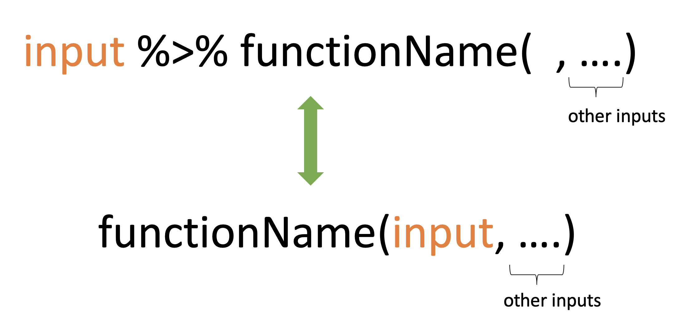 --- ## Built-in dataset ```r library(palmerpenguins) data(penguins) head(penguins) ``` ``` # A tibble: 6 × 8 species island bill_length_mm bill_depth_mm flipper_length_… body_mass_g sex <fct> <fct> <dbl> <dbl> <int> <int> <fct> 1 Adelie Torge… 39.1 18.7 181 3750 male 2 Adelie Torge… 39.5 17.4 186 3800 fema… 3 Adelie Torge… 40.3 18 195 3250 fema… 4 Adelie Torge… NA NA NA NA <NA> 5 Adelie Torge… 36.7 19.3 193 3450 fema… 6 Adelie Torge… 39.3 20.6 190 3650 male # … with 1 more variable: year <int> ``` --- ## Skim data ```r library(skimr) skim(penguins) ``` --- ## iris dataset 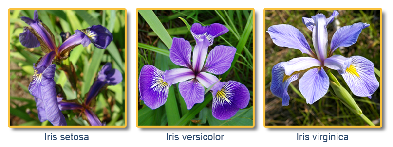 --- 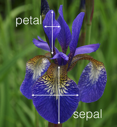 --- Use the R dataset “iris” to answer the following questions: 1. How many rows and columns does iris have? 2. Select the first 4 rows. 3. Select the last 6 rows. 4. Select rows 10 to 20, with all columns in the iris dataset. 5. Select rows 10 to 20 with only the Species, Petal.Width and Petal.Length. 6. Create a single vector (a new object) called ‘width’ that is the Sepal.Width column of iris. 7. What are the column names and data types of the different columns in iris? 8. How many rows in the iris dataset have `Petal.Length` larger than 5 and `Sepal.Width` smaller than 3? <div class="countdown" id="timer_62133dbf" style="right:0;bottom:0;" data-warnwhen="0"> <code class="countdown-time"><span class="countdown-digits minutes">05</span><span class="countdown-digits colon">:</span><span class="countdown-digits seconds">00</span></code> </div> --- class: inverse, cover, middle # Recap ✅ Data structures and functions ✅ Factors ✅ Working with packages ✅ Create a tibble ✅ Help file ✅ Commenting